The Application of the Technology of 3D Satellite Cloud Image in Virtual Reality Simulation
XIE Xiao-fang 1, QIAO Yong-jun 2, Sun Tao 3
1 Department of Ordnance Science and Technology, Naval Aeronautical Engineering Institute, Yantai 264001, China
2, 3 Graduate Students' Brigade of Naval Aeronautical Engineering Institute, Yantai 264001, China
Abstract
Using satellite cloud image to simulate cloud is one of the new visual simulation technologies adopted in Virtual Reality (VR). Taking the original data of satellite cloud images as the source, this paper depicts specifically the technology of 3D satellite cloud image through the transforming of coordinates and projection, creating DEM of cloud image and 3D simulating. To create cloud image DEM, Mercator projection was introduced to create regular cloud image grid, while solutions for geodetic problems was introduced to calculate distance, and the outer-trajectory science of rocket was introduced to get the elevation of cloud. For demonstration, we use Microsoft Visual C++ and OpenGL to simulate the 3D satellite cloud image.
Keywords
virtual reality; satellite cloud image; projection transformation; cloud image DEM; three-dimension simulation
1 Introduction
With the technology of Synthetic Environment (SE) based on real natural environment being widely employed in VR, more detailed environment data is required for the visual simulation. As the most convenient and available data source, satellite cloud image has enormous potential to explore. Figure 1 shows the usual application flow.
 |
Fig.1 Usual application flow
2 Projection Transformation of Satellite Cloud Image
The cloud image abstracted from original data is an image of global disk, it is 2048×2048 in dimension. Because the disk image is an inextensible spherical surface, and the scale in different area is different, thus, it must be projected into a square image by transformation. Projection transformation is to establish the functional relations between geographical coordinates and Cartesian coordinates, it can be formulated as
x = f1(L, B) y = f2(L, B) (1)
Where (x, y) is the Cartesian coordinates, (L, B) is the geographical coordinates.
Above formulas are the general equations of projection transformation, for different projection, the expressions of f1 and f2 differ accordingly.
2.1 Calculating the Geographic Coordinates
Other than common projection, the geographic coordinates of a point in disk image is unknown, so we must get its geographic coordinates before the projection.
Using the information of location, we can get the number of the first scan line, the pixel number of the first scan column, together with the numbers of scan lines and the numbers of pixels in 25 by 25 lattice. By virtue of these data, we can calculate the geographic coordinates and pixel coordinates of every point within lattice. Every point doesn’t belong to lattice must be in a quadrangle whose vertexes are four points in lattice. Thus, the geographic coordinates of this point can be expressed by the coordinates of these four points. Because the space between two grids is small, the longitude or latitude can be regarded as a beeline. In this quadrangle, let the geographic coordinates of Ai (Bi, Li), Ai is one of clockwise four vertexes, its pixel coordinates is (xi, yi), then the geographic coordinates (Bp, Lp) of a point in this quadrangle is
![]() (2)
(2)
Where i and j are the roots of the following equations
 (3)
(3)
This method is faster and more precise than the method of line and row scanning.
2.2 Projection Transformation
In the transformation between Cartesian coordinates and geographic coordinates, projection plays an important role. The common projections of satellite cloud image include Mercator cylindrical projection, Lambert conic projection, Stereographic projection, Gauss-Krüger projection and etc. In these projections, Mercator cylindrical projection has valuable characteristics that the grid composed of longitudes or latitudes is a rectangle after projection, which is suitable for creating cloud image DEM. Moreover, just because the image projected is a rectangle, it is easy to joint several cloud images into a big one.
Fig.2 Mercator projection
Figure 2 illustrates the Mercator projection of satellite cloud image. After the projection, the point A, B, C, D and P were mapped into the point A′, B′, C′, D′ and P′. Where A and B, C and D are in the same latitude respectively. Besides, A and D, B and C are in the same longitude respectively. According to the principle of projection, the corresponding points will still in the same longitudes and latitudes. The relation of Point P and point P′ is
 (4)
(4)
Projection transformation is to map P to P′, the inverse transformation is to map P′ to P. Here, we use reverse transformation, for it assure the surjection, so we needn’t interpolate after the projection. Meanwhile, we can calculate variables i and j conveniently by the interpolation.
Under Visual C++, assume variable grid is a CPoint pointer, it points to the pixel coordinates array of 24 by 24 lattice, then the mapping between P(X, Y) and P′(B, L) can be expressed as follows:
i = 0.2 * (5 – B + (int)B / 5 * 5);
if (L > 0) {
j = 0.2 * (L - (int)L / 5 * 5);
if (j < 1.0E6) j = 1;
}
else {
j = 0.2 * (5 + L - (int)L / 5 * 5);
}
X = i * j * grid[g y* 25 + gx].x + (1 - i) * j * grid[gy * 25 + gx + 1].x
+ i * (1 - j) * grid[gy * 25 + gx + 25].x + (1 – i – j + i * j) grid[gy * 25 + gx + 26].x;
Y = i * j * grid[gy * 25 + gx].y + (1 - i) * j * grid[gy * 25 + gx + 1].y
+ i * (1 - j) * grid[gy * 25 + gx + 25].y + (1 – i – j + i * j) grid[gy * 25 + gx + 26].y;
Where gx and gy are the grid coordinates that the point P′(B, L) in. Figure 3 is one part of the satellite cloud image after Mercator projection used with the above method.
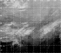
Fig.3 The satellite cloud image after Mercator projection
3 Creating of Satellite Cloud Image DEM
As one kind of simulation model, Digital Elevation Model (DEM) is widely used in Geographical Information Systems (GIS) and VR. After the Mercator projection and data sampling with certain sample space in conformity to resolution, we get the data grid, together with the elevation, finally we get the DEM of satellite cloud image.
3.1 Distance Solution of Satellite Cloud Image
Because the cloud image DEM satisfied the standards of USGU DEM, first we must calculate the distance of two points A(B1, L1) and B(B2, L2) in the satellite cloud image. The distance can be solved by the method of solutions of geodetic problems.
Before the distance solution, we should convert the parameter B1, L1, B2 and L2 into radian.
b = B2 - B1
P = sinb·cosL2
Q = cosL1·sinL2 - sinL1·cosL2·cosb
M = sinL1·sinL2 + cosL1·cosL2·cosb
A0 = atan( P / Q )
A1 = atan(cosL2·sinA0 / sqrt(1 - cosL2·sinA0·cosL2·sinA0))
A = atan((P·sinA0 + Q·cosA0) / M)
S = 6356863.020 + (10708.949 - 13.474cosA1)cosA1
L = A·S
Here variable L is the distance required, all other variables such as b, P are temporary variables, the constant are the elements of the Krasovsky ellipsoid.
3.2 Calculation of Elevation
The elevation of cloud can be calculated by the infrared and visible light criteria in the information of criteria. These criteria are bright temperature and albedo. Take the bright temperature for example, the satellite cloud image is composed of 256 grey levels, through the transformation of bright temperature, every grey level can be converted into the corresponding temperature. If the location that simulated is above cloud, we can just select a camber datum, thus according to the temperature variation law with the altitude, we can calculate the relative altitude, namely, it expresses the elevation of every piece of cloud as relative altitude. If the viewpoint is variable, we must calculate the absolute altitude. As the precondition, we must get the corresponding temperature of ground surface and the altitude of the bottom of cloud, which all can be gotten from the live meteorological data. With these data, we can create not only the cambered model of cloud, but also the closed-curve surface model of the body of cloud.
Because the law that temperature varies with the altitude is different in the different area, even for the same area, it also changes with time. To achieve higher simulation precision, here we use the outer-trajectory science of rocket for reference to calculate the elevation of cloud.
Under the standardized atmosphere and standardized meteorological condition, the standard law of virtual temperature varies with altitude is
![]() (5)
(5)
Where τon=288.9K, G1=6.328×10⁻³K/m, Z is the altitude.
The transition formula of virtual temperature τ(Z) and air temperature t(Z) is
 (6)
(6)
Where p(Z) is the overall pressure of humid air, a(Z) is the component of vapor (i.e. absolute humidity).
The meteorological condition is different in troposphere and stratosphere, so we should make a difference between them.
 (7)
(7)
In the above formula, the constant G=B=6.328×10⁻³ K/m, A=230.0K, C=1.172×10⁻⁶ K/m2.
Above formula is the form of standard meteorological condition, where virtual temperature is the standard virtual temperature. In practical application, they should be amended according to the real ground observation.
![]() (8)
(8)
Let Z = 0, then τd = τ(0) - τon, with p(0) and a(0), we can calculate the τ(0). Thus, after converting the temperature of the top of cloud to virtual temperature, inverse calculation will result in the more precise altitude of cloud.
4 Simulation of 3D Satellite Cloud Image
Nowadays, there are main four methods to simulate cloud in VR visual simulation. The first and simplest step is to fill the sky with blue. The second step is BOX, i.e. mapping texture on polygon. The third one is DOME, it looks the sky as a half sphere and map texture on its surface. The last method introduces a sky model with seven layers, they are the top thin cloud layer, the cloud layer, the bottom cloud layer, and so on. For these layers, according to their height and brightness, we can map the corresponding texture on it.
The common characteristics of above method is that they are all use the technology of texture mapping, the cloud simulated is not the real cloud on the real time, so they can’t simulate the real cloud with 3D structure.
Here, we introduce a DEM method to simulate the real cloud. Since the satellite cloud image is represented with the color, so color render is better than texture mapping. To create 3D satellite cloud image, we can use many methods such Bezier camber and Nurbs camber based on OpenGL.
Figure 4 is the 3D satellite cloud image created in Visual C++. The first step is curve interpolation on DEM data, the second one is triangular approximation, and the last one is color rendering. Having DEM, we can also convert it into another 3D model in Open Flight format with the software Multigen Creator, thus we can just use it as an object in software Multigen Vega.
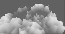
Fig.4 The 3D satellite cloud image created in Visual C++
The following C++ function is the instance to create 3D satellite cloud image based on OpenGL. In this function, we put many 3-order Bezier cambers together to create the full image. Suppose the mesh after sampling is an M by N grid, the horizontal and vertical width of cells are xStride and yStride respectively, while the number of cells is xNum and yNum, variable order is the order of camber, pointer grid points to the data of elevation of image.
void Draw3DCloud( )
{
float x,y,z;
static float ctrlpoints[4][4][3];
for(int i=0; i<(M-1)/order; i++)
for(int j=0;j<(N-1)/order;j++){
for(int k=0;k<(N-1)/order;k++)
for(int l=0;l<=order;l++){
x=(i*order+k)*xStride;
z=(j*order+l)*yStride;
y=grid[(j*oem+1)*M+i*order+k];
ctrlpoints[k][l][0]=x;
ctrlpoints[k][l][1]=y;
ctrlpoints[k][l][2]=z;
}
glMap2f(GL_MAP2_VERTEX_3,0,1,3,order+1,0,1,12,order+1,&ctrlpoints[0][0][0]);
glEvalMesh2(GL_FILL,0,xNum,0,yNum);
}
}
5 Conclusion
The method introduced above has achieved good visual simulation effects, which is of important applicable value in military VR and has been applied to the pre-research project of the “Tenth Five-Year-Plan” of China. The data of Satellite cloud image is very dense and timely, so it can be applied to improve the simulation precision, thus it can be a new data source for visual simulation and military application. A fly in the ointment, the calculation of elevation of cloud image DEM depends on the statistical model.
Acknowledgement
This work was supported by the Military Grand Laboratory Foundation of China under Grant No.2110-11-201.
We thank Prof. Liu Ai-dong and Dr. Wang Chang-jin for their comments and suggestions.
References
[1] Xie Xiaofang. The technology of virtual reality and its application. Beijing: Haichao Publishing House, 2002. 1-6
[2] Wang Wenjun. The second developing of WT-8D Geostationary Meteorological Satellite Data Processing System. Militray meteorology, 2002. (1) : 39
[3] Hua Yixin, Wu Sheng, Zhao Junxi. The principle and technology of Geographical Information System. Beijing: Liberation Army Publishing House, 2001. 85-96
[4] Standards for Digital Elevation Models. U.S. Department of the Interior U.S. Geological Survey National Mapping Division, 1992. 2_21-2_37
[5] Kong Xiangyuan, Mei Shiyi. Control Surveying. Wuhan: Wuhan Technical University of Surveying & Mapping Press, 1998. 43-53
[6] Xi Mingyou. Outer- trajectory science of rocket. Beijing: The Publishing House of Ordnance Industry, 1989. 10-15
[7] Wu Yunlong, Zhang Yunmeng, Xu Gang. The theory of accuracy parameter of self-propelled antiaircraft gun weapon system. Beijing: The Publishing House of National Defence Industry, 1999. 88-90
[8] Zhao Qinping. DVENET distributed virtual environment. Beijing: Science Press, 2002. 114-136
[9] Zhang Xiushan. The technology of virtual reality and the technique of programming. Beijing: University of National Defence Technology Press, 1999. 163-173
Brief introduction of authors
Mr. XIE Xiao-Fang was born in 1962. He is a professor and doctoral supervisor at the Naval Aeronautical Engineering Institute. His researches areas are fire control and virtual reality.
e-mail: xiexf106@yahoo.com.cn
tel: +86 05356635583, +86 13505357438
Mr. QIAO Yong-Jun was born in 1974. He is a engineer and Ph.D. candidate at the Naval Aeronautical Engineering Institute. His current research interests are virtual reality and modeling & simulation of weapon system.
e-mail: qyjdatabase@163.com
tel: +86 05356230064, +86 13002757080
Mr. SUN Tao was born in 1980. He is a Ph.D. candidate at the Naval Aeronautical Engineering Institute. His current research interest is the technology of missile breaking through defense and countermeasure.
tel: +86 05356635586, +86 13583555117